library(leaflet)
leaflet() |>
  addTiles() |>   # Add default OpenStreetMap map tiles
  addMarkers(lat = 38.90243843683386, lng =  -77.0443814477152,
label = "Elliott School of International Affairs")R and RStudio Setup
Packages in this module
Packages: tidyverse, leaflet, vdemlite, unvotes
R and RStudio
All of our work for this course will be done in the R language and we will be working with R in RStudio. RStudio is an integrated development environment (IDE) develop by a company named Posit. Please be sure to download and install the most recent versions of R and R Studio from Posit’s website.
It is a good idea to periodically update R and RStudio. RStudio will prompt you when it is time to update and you can follow the same process of downloading and installing from the Posit website that we just did here. For R, the easiest approach is to use rig (R Installation Manager), which works on Windows, Mac, and Linux and lets you install and switch between R versions from the command line. On Windows you can also use the installr package. I usually update R once a semester.
We are going to be using a number of R packages throughout the course. One essential set of packages are those that comprise the Tidyverse, but especially readr, dplyr, ggplot2 and tidyr. You can install the entire Tidyverse collection of packages by typing install.packages("tidyverse") in your console. We will talk about these packages in detail as we go through the course, but have a look at this basic description now to gain some basic familiarity.
Another thing that you really want to do is to make sure that you have the native pipe operator (|>) enabled. In RStudio, go to Tools>Global Options, then go to Code and select “Use native pipe operator.”
While you are here, you can also go to Appearance to select a different editor theme or to Pane Layout to change how the four panes in R Studio are organized. Next, familiarize yourself with how to expand and minimize the four windows. The most important window that I want to highlight here is the source window. This is where we are going to be working most of the time in this course. And if I tell you to send your source code, I mean to send the file that you are working on in this window. This could be a Quarto document, an R script or an app.R file for a Shiny app.
The next window is the Console and there we also see tabs for Terminal and Background Jobs. The console is where you can run R code one line at a time. The terminal is relevant for more advanced users and we will make some use of it when we talk about publishing Quarto documents. Background Jobs is going to be helpful when we want troubleshoot a Quarto document that is not rendering properly.
From there, the next pane we want to explore is Environment, History, etc. Environment tells us what files are currently available to us.
Finally, we see a pane with Files, Plots, Packages etc. Files tells us what files are in our project folder and enables us to copy, and delete files associated with our project. Plots is a window for viewing our visualizations. And Packages shows us what packages are available and loaded into our environment.
Before you move on to the next section, take some time to familiarize yourself with the various user-friendly buttons and shortcuts available to you like the drop down menu for the pane layout, a spell checker, a button for inserting a code chunk and other features that you can play around with.
Three Visualization Examples
Now that RStudio is set up, let’s get our hands dirty by running some real data visualization code. The three examples below use packages we will cover in much more depth as the course goes on, but for now the goal is just to run the code, render the document, and see what R can do.
Create a new Quarto document, copy each code chunk below into it, and render. Try tweaking small things (a country name, a color, a date range) and re-render to see what changes.
Example 1: Make a Map!
Example 2: Plotting Democracy Over Time
# Load the packages
library(vdemlite)
library(ggplot2)

# Use vdemlite to extract democracy scores for France and India
dem_data <- fetchdem(indicators = "v2x_polyarchy",
                     countries = c("FRA", "IND"))

# And now we can plot the data
ggplot(dem_data, aes(y = v2x_polyarchy, x = year, color = country_name)) +
  geom_line() +
  theme_minimal() +
  xlab("Year") +
  ylab("Electoral Democracy Index") +
  ggtitle("Electoral Democracy, 1970-2022") +
  geom_hline(yintercept = .5, linetype = "dashed", color = "grey") +
  scale_color_manual(name = "Country", values = c("#E69F00", "#56B4E9")) +
  ylim(0, 1)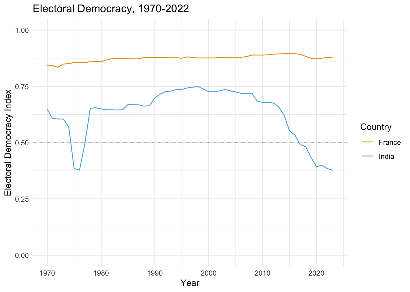
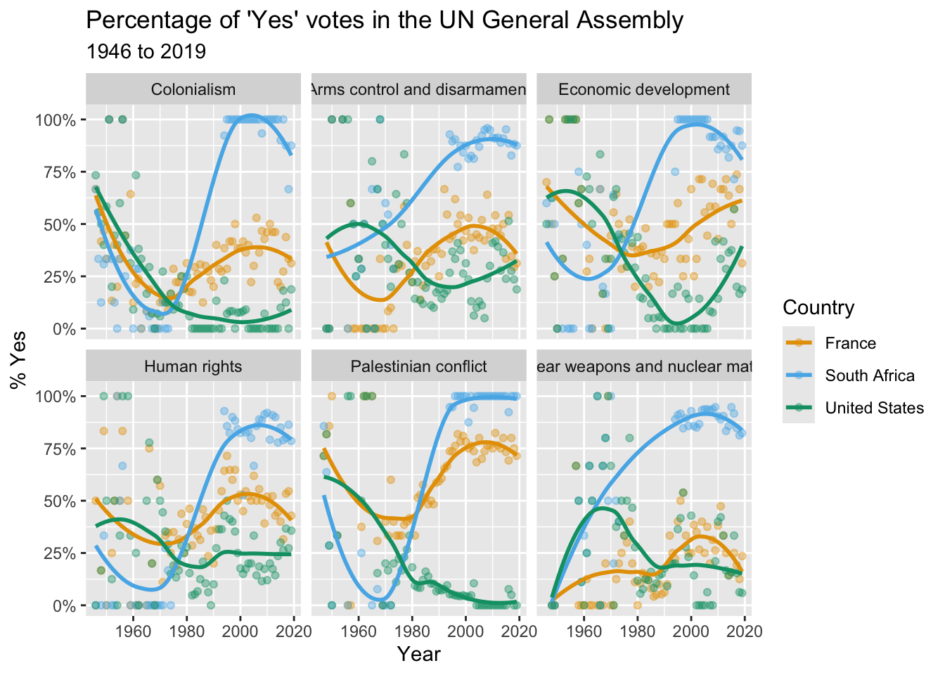
Example 3: UN Voting Trends
library(tidyverse)
library(unvotes)
library(lubridate)
library(scales)
library(pacman)

unvotes <- un_votes |>
  inner_join(un_roll_calls, by = "rcid") |>
  inner_join(un_roll_call_issues, by = "rcid")

unvotes |>
  # then filter out to only include the countries we want
  filter(country %in% c("South Africa", "United States", "France")) |>
  # then make sure R understands the the year variable is a date
  mutate(year = year(date)) |>
  # Then group the data by country and year
  group_by(country, year, issue) |>
  # then take the average Yes votes for each country_year
  summarize(percent_yes = mean(vote == "yes")) |>
  # then make a nice plot
  ggplot(mapping = aes(x = year, y = percent_yes, color = country)) +
  geom_point(alpha = 0.4) +
  geom_smooth(method = "loess", se = FALSE) +
  facet_wrap(~issue) +
  scale_y_continuous(labels = percent) +
  scale_color_manual(values = c("#E69F00", "#56B4E9", "#009E73")) +
  labs(
    title = "Percentage of 'Yes' votes in the UN General Assembly",
    subtitle = "1946 to 2019",
    y = "% Yes",
    x = "Year",
    color = "Country"
  )