library(peacesciencer)
library(dplyr)

conflict_df <- create_stateyears(system = 'gw') |>
  filter(year %in% c(1946:1999)) |>
  add_ucdp_acd(type=c("intrastate"), only_wars = FALSE) |>
  add_democracy() |>
  add_creg_fractionalization() |>
  add_sim_gdp_pop() |>
  add_rugged_terrain() |>
  mutate(gdppc = log(mrgdppc), # log GDP per capita
         pop = log(pwtpop))    # log population

glimpse(conflict_df)Regression Tables
November 3, 2026
What’s in a Regression Table?
Load Data
Run Model
View with summary()
Call:
glm(formula = ucdponset ~ ethfrac + relfrac + v2x_polyarchy +
    rugged + gdppc + pop, family = binomial(link = "logit"),
    data = conflict_df)

Coefficients:
              Estimate Std. Error z value Pr(>|z|)
(Intercept)   -1.62860    0.99050  -1.644  0.10013
ethfrac        0.71013    0.37159   1.911  0.05600 .
relfrac       -0.24805    0.40739  -0.609  0.54260
v2x_polyarchy -0.73674    0.50941  -1.446  0.14810
rugged         0.08712    0.07567   1.151  0.24959
gdppc         -0.37570    0.11969  -3.139  0.00169 **
pop            0.29367    0.06866   4.277 1.89e-05 ***
---
Signif. codes:  0 '***' 0.001 '**' 0.01 '*' 0.05 '.' 0.1 ' ' 1

(Dispersion parameter for binomial family taken to be 1)

    Null deviance: 1205.0  on 6128  degrees of freedom
Residual deviance: 1148.6  on 6122  degrees of freedom
  (1495 observations deleted due to missingness)
AIC: 1162.6

Number of Fisher Scoring iterations: 7
View results with broom
# A tibble: 7 × 7
  term          estimate std.error statistic p.value conf.low conf.high
  <chr>            <dbl>     <dbl>     <dbl>   <dbl>    <dbl>     <dbl>
1 (Intercept)    -1.63      0.990     -1.64  0.100   -3.56        0.326
2 ethfrac         0.710     0.372      1.91  0.056   -0.00629     1.45
3 relfrac        -0.248     0.407     -0.609 0.543   -1.05        0.547
4 v2x_polyarchy  -0.737     0.509     -1.45  0.148   -1.75        0.252
5 rugged          0.0871    0.0757     1.15  0.250   -0.0680      0.229
6 gdppc          -0.376     0.120     -3.14  0.00169 -0.615      -0.146
7 pop             0.294     0.0687     4.28  0.00002  0.160       0.430
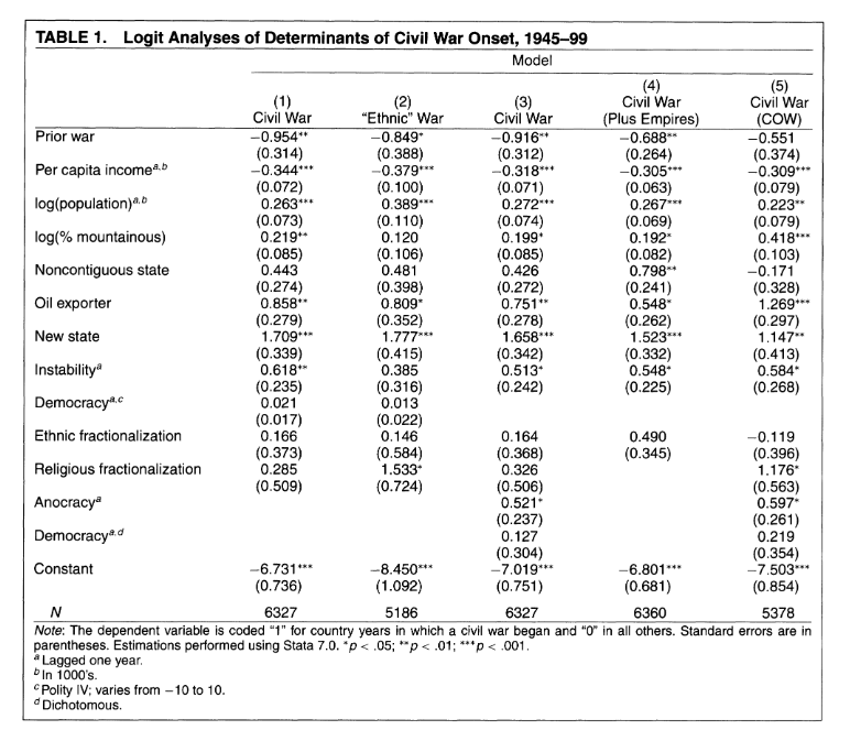
How close are our results to F&L?
Discuss with a neighbor…
# A tibble: 7 × 7
  term          estimate std.error statistic p.value conf.low conf.high
  <chr>            <dbl>     <dbl>     <dbl>   <dbl>    <dbl>     <dbl>
1 (Intercept)    -1.63      0.990     -1.64  0.100   -3.56        0.326
2 ethfrac         0.710     0.372      1.91  0.056   -0.00629     1.45
3 relfrac        -0.248     0.407     -0.609 0.543   -1.05        0.547
4 v2x_polyarchy  -0.737     0.509     -1.45  0.148   -1.75        0.252
5 rugged          0.0871    0.0757     1.15  0.250   -0.0680      0.229
6 gdppc          -0.376     0.120     -3.14  0.00169 -0.615      -0.146
7 pop             0.294     0.0687     4.28  0.00002  0.160       0.430
Could we get closer to F&L?
- How close are our data to F&L’s?
- Got to the peacesciencer documentation
- Could we change something to better approximate their results?
- Are there predictors in the
peacesciencerpackage that were not available to F&L?
Regression Tables with modelsummary
- Oftentimes we want to show multiple models at once (like F&L)
- We want to compare across them and see which is the best model
- How can we do that?
- There are many ways to do this in R
- We will use the
modelsummarypackage
Run Multiple Models
ethnicity <- glm(ucdponset ~ ethfrac + relfrac + gdppc + pop, # store each model in an object
                  data = conflict_df,
                  family = "binomial")

democracy <- glm(ucdponset ~ v2x_polyarchy + gdppc +  pop,
                  data = conflict_df,
                  family = "binomial")

terrain <- glm(ucdponset ~ rugged + gdppc + pop ,
                  data = conflict_df,
                  family = "binomial")

full_model <- glm(ucdponset ~ ethfrac + relfrac + v2x_polyarchy + rugged +
                        gdppc + pop,
                  data = conflict_df,
                  family = "binomial")
Prep Data for Display
models <- list("Ethnicity" = ethnicity,  # store list of models in an object
               "Democracy" = democracy,
               "Terrain" = terrain,
               "Full Model" = full_model)

coef_map <- c("ethfrac" = "Ethnic Frac",  # map coefficients
        "relfrac" = "Religions Frac",     #(change names and order)
        "v2x_polyarchy" = "Polyarchy",
        "rugged" = "Terrain",
        "gdppc" = "Per capita GDP",
        "pop" = "Population",
        "(Intercept)" = "Intercept")

caption = "Table 1: Predictors of Conflict Onset" # store caption
reference = "See appendix for data sources."      # store reference notes
Display the Models
Code
| Ethnicity | Democracy | Terrain | Full Model | |
|---|---|---|---|---|
| + p < 0.1, * p < 0.05, ** p < 0.01, *** p < 0.001 | ||||
| See appendix for data sources. | ||||
| Ethnic Frac | 0.747* | 0.710+ | ||
| (0.364) | (0.372) | |||
| Religions Frac | -0.373 | -0.248 | ||
| (0.406) | (0.407) | |||
| Polyarchy | -0.349 | -0.737 | ||
| (0.436) | (0.509) | |||
| Terrain | 0.036 | 0.087 | ||
| (0.075) | (0.076) | |||
| Per capita GDP | -0.478*** | -0.497*** | -0.539*** | -0.376** |
| (0.104) | (0.105) | (0.092) | (0.120) | |
| Population | 0.290*** | 0.302*** | 0.303*** | 0.294*** |
| (0.068) | (0.051) | (0.050) | (0.069) | |
| Intercept | -0.887 | -0.425 | -0.254 | -1.629 |
| (0.898) | (0.791) | (0.758) | (0.991) | |
| Num.Obs. | 6364 | 6955 | 6840 | 6129 |
Your Turn!
- Got to the peacesciencer documentation
- How close are our data to F&L’s?
- Could we change something to better approximate their results?
- Run multiple models using different predictors
- Display the models using
modelsummary - Try to get as close to F&L as you can!
Coefficient Plots
This doesn’t look that great…
Show the code
| (1) | |
|---|---|
| + p < 0.1, * p < 0.05, ** p < 0.01, *** p < 0.001 | |
| See appendix for data sources. | |
| Ethnic Frac | 0.710+ |
| (0.372) | |
| Religions Frac | -0.248 |
| (0.407) | |
| Polyarchy | -0.737 |
| (0.509) | |
| Terrain | 0.087 |
| (0.076) | |
| Per capita GDP | -0.376** |
| (0.120) | |
| Population | 0.294*** |
| (0.069) | |
| Intercept | -1.629 |
| (0.991) | |
| Num.Obs. | 6129 |
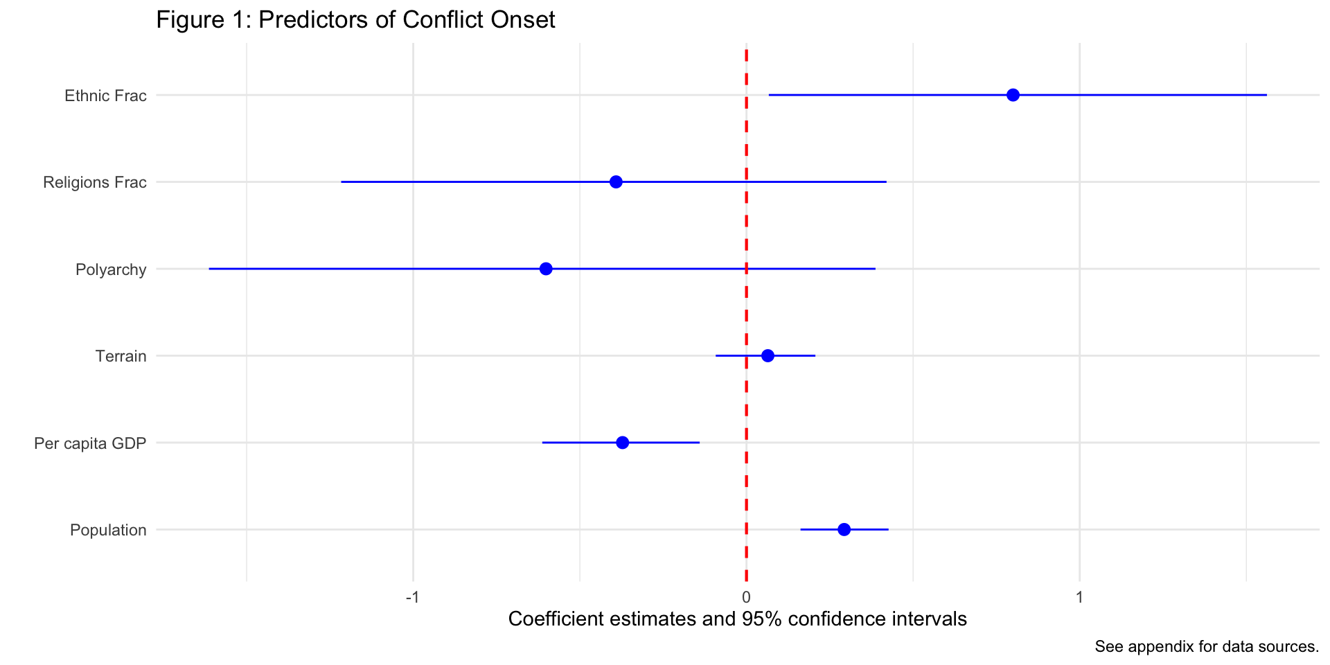
So we can use ggplot to make a coefficient plot instead…
Show the code
library(ggplot2)

modelplot(conflict_model,
          coef_map = rev(coef_map), # rev() reverses list order
          coef_omit = "Intercept",
          color = "blue") + # use plus to add customizations like any ggplot object
  geom_vline(xintercept = 0, color = "red", linetype = "dashed", linewidth = .75) + # red 0 line
  labs(
    title = "Figure 1: Predictors of Conflict Onset",
    caption = "See appendix for data sources."
) 
Your Turn!
- Take one of your models
- Use
modelplotto create a coefficient plot of it - Customize the plot to your liking
- Interpret the results
- Discuss advantages of coefficient plots with a neighbor